Guide for creating plot boundaries in PlantCV-Geospatial¶

Here we provide some suggestions on how to outline your individual plants or plots depending on your planting strategy. If this is your first time using PlantCV-Geospatial, we recommend checking out our Getting Started guide first!

Table of contents¶

1. Field layout vocabulary
2. Individual plants
   • In a grid
   • Irregular spacing
3. Row crops
   • Precision planted
   • Irregular spacing
4. Isolated plots

Field layout vocabulary
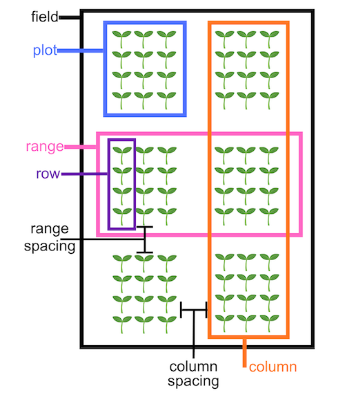
Several plot boundary creation tools in PlantCV-Geospatial rely on named parameters that follow a consistent way of describing how you might layout a field experiment. Refer to the diagram below for the common terms. Because of the transformation from latitude and longitude, your field might be tilted, so the designation of range vs column is relative to the top left corner of the field. PlantCV-Geospatial has a Field_layout class designed to keep track of these parameters. We recommend filling this out at the beginning of your notebook.

# A notebook for field analysis

# Imports
%matplotlib widget
import plantcv.plantcv as pcv
import plantcv.geospatial as gcv

pcv.params.debug = "plot"

# Fill out experimental details - in meters
gcv.field_layout.num_ranges=9
gcv.field_layout.num_columns=9
gcv.field_layout.range_length=0.74
gcv.field_layout.row_length=0.76
gcv.field_layout.num_rows=1
gcv.field_layout.range_spacing=0
gcv.field_layout.column_spacing=0

Individual plants
Your experimental units might be individual plants, like this:

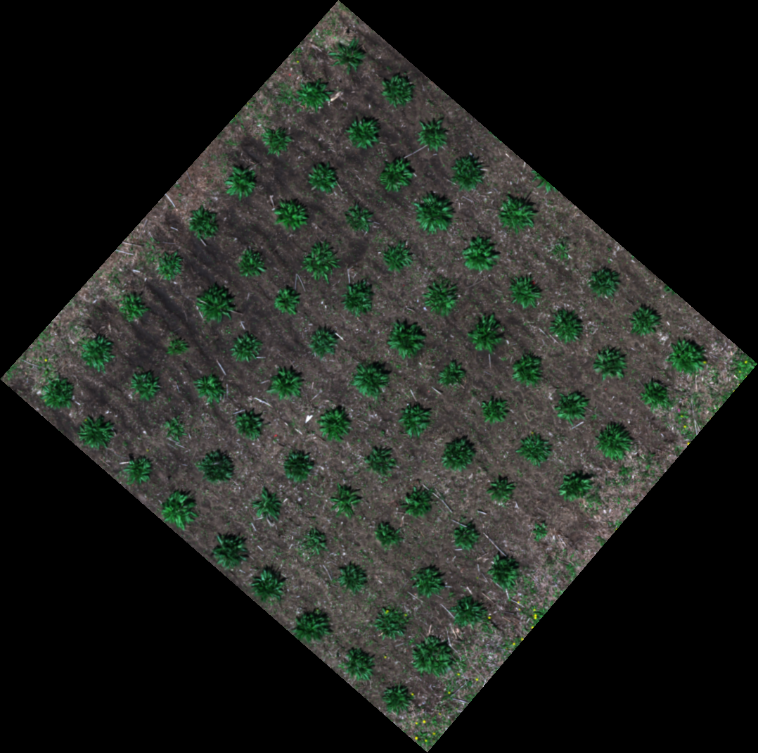
• In a grid - If your individual plants are in a relatively uniform grid, like the example above, you should first try the most automated of PlantCV-Geospatial's plot boundary creation methods, create_shapes.auto_grid, which accounts for the attributes of field_layout to create and save a grid of plot boundaries.

# Other parameters are taken automatically from field_layout if you have filled it in
gcv.create_shapes.auto_grid(img, cropto="./field_corners.geojson", outpath="./plots.geojson")

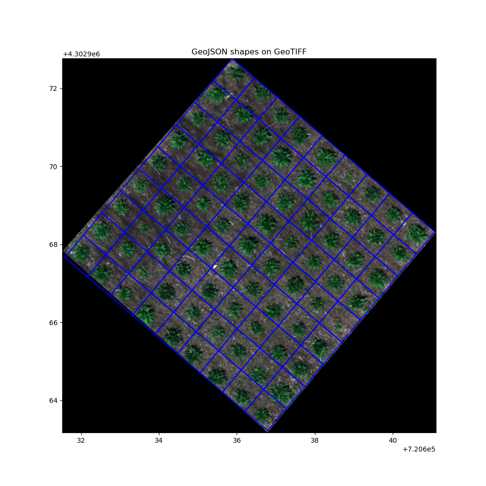
• Irregularly spaced - If your individual plants are planted less uniformly, and you need the flexibility to modify the grid, PlantCV-Geospatial provides a set of steps that automatically create shapes, but give you the chance to manual change them in between steps to fit around your plants. See the docs for the InteractiveShapes class for more about how this works. Briefly, you will open an interactive window where you will draw a box around your field. Then, lines will be automatically drawn forming a grid with your field dimensions (number of ranges x number of columns). You can manually move the lines until you are satisfied with their positions relative to your plants. Finally, polygons will be automatically drawn using the intersection of the grid lines. You can again manually change the position of the polygons until you are satisfied, at which point you can save the shapes to a geojson that can be used for analysis.

Row crops
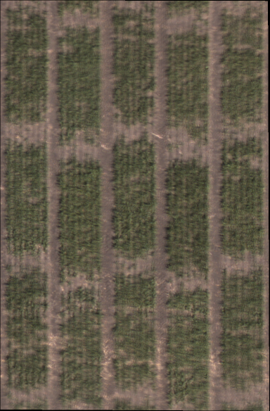
Especially in systems like small grains, your experimental units might be plots composed of rows of the same genotype or treatment. Example images below are from the Bison-Fly: UAV pipeline at NDSU Spring Wheat Breeding Program.

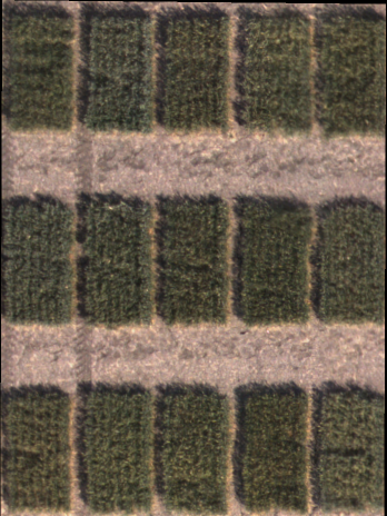
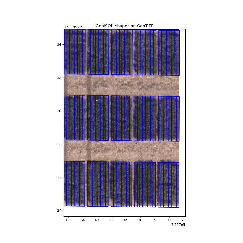
• Precision planted - Precision planters can result in fields where plots are predictably spaced with evenly-spaced alleyways between ranges and columns. In this case, the automatic grid approach described above for single plants can work well:

gcv.field_layout.num_ranges=3
gcv.field_layout.num_columns=5
gcv.field_layout.range_length=2.7
gcv.field_layout.row_length=0.18
gcv.field_layout.num_rows=8
gcv.field_layout.range_spacing=1.28
gcv.field_layout.column_spacing=0.195

gcv.create_shapes.auto_grid(img, cropto="./field_corners.geojson", outpath="./plots.geojson")

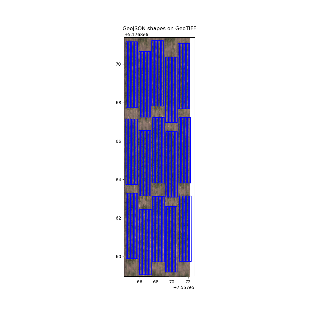
• Irregular spacing - If your row crops are less precisely planted, PlantCV-Geospatial has a more manual plot boundary creation method, create_shapes.grid_from_coords that uses points you provide describing where the corners of each plot are. This information is in a points-type geojson shapefile created by clicking on the top corner of each plot. This file can be made in a separate program, like QGIS, or using the add_layer and to_points methods of an InteractiveShapes class object. See an example in the docs here.

gcv.field_layout.range_length=3.4
gcv.field_layout.row_length=0.18
gcv.field_layout.num_rows=8

gcv.create_shapes.grid_from_coords(img, field_corners_path="./field_corners.geojson", 
                                   plot_geojson_path="./plot_corners.geojson", out_path="./plots.geojson)

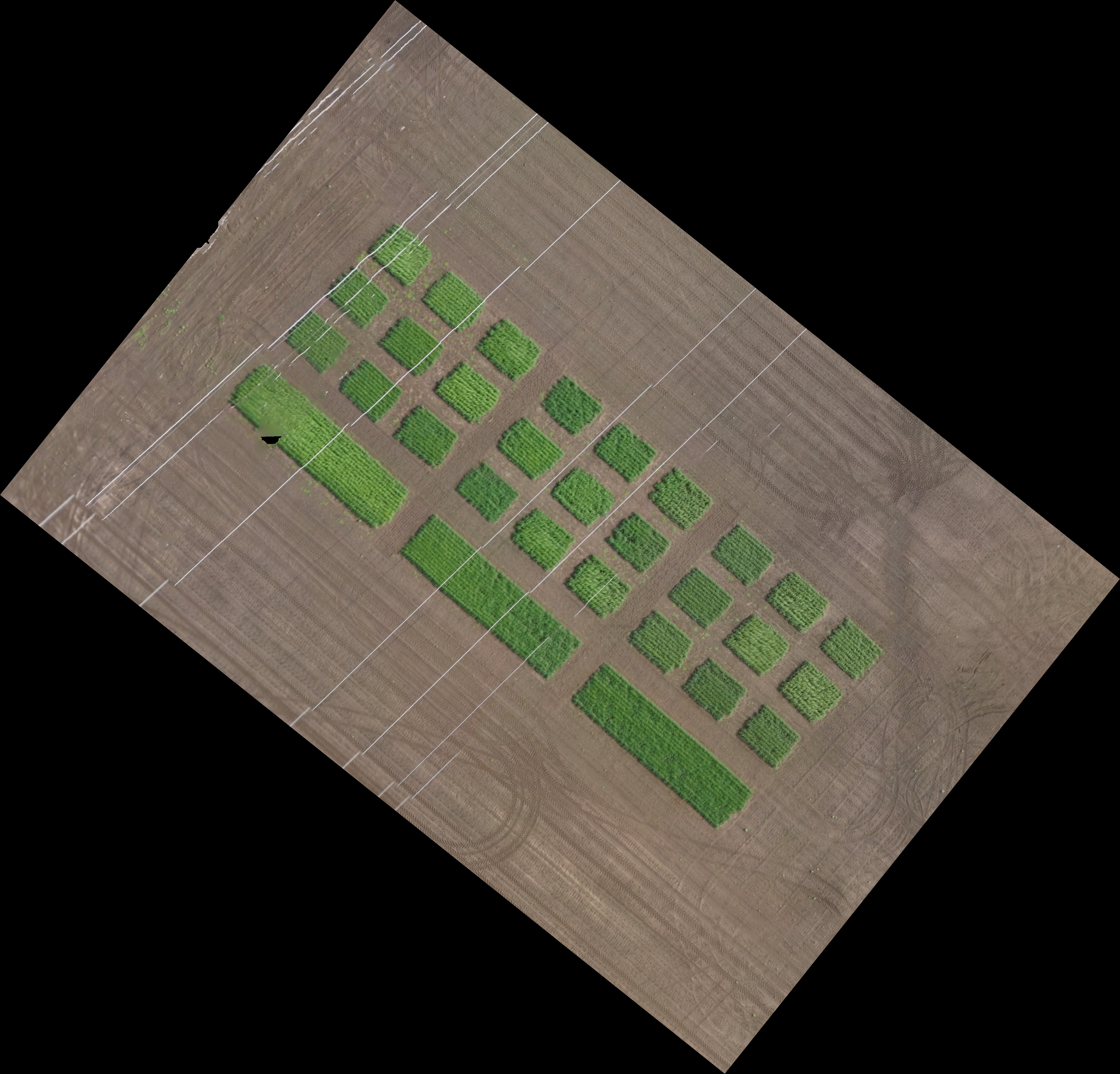
Isolated plots
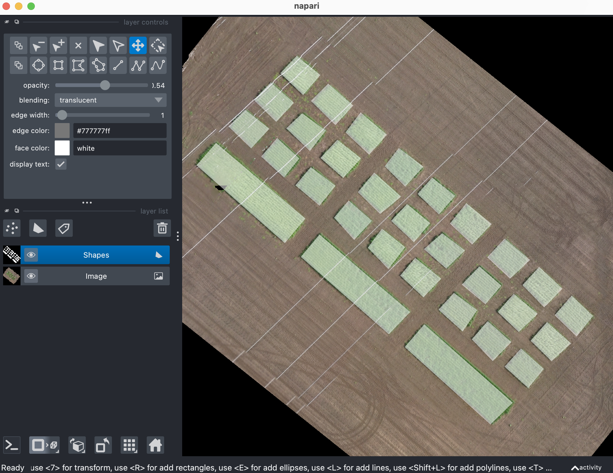
If you instead have few, disjointed or randomly placed single plants or row plots that might be far apart, more manual plot boundary creation methods might end up being easier or faster. Because the InteractiveShapes class opens an interactive viewer, it is possible to add custom shapes that fit any field that can be directly saved to a geojson for use in analysis functions.

Example images below from Brown, K. E., Schuhl, H., Srivastava, D., Beyene, G., Li, M., Fahlgren, N., & Murphy, K. M. (2026). Quantifying growth and lodging in Tef (Eragrostis tef) with Uncrewed Aerial Systems (UAS). bioRxiv, 2026-01.

geotif = "./isolated_plots.tif"
cropto = "./crop.geojson"


img = gcv.read.geotif(geotif, bands="b,g,r", cropto=cropto)
editor = gcv.create_shapes.InteractiveShapes(img)
editor.add_layer(layer_type="shapes")

After adding your shapes using the polygon drawing tool:

And finally, save the shapes in the next cell:

editor.to_shapes(dest="./plots.geojson", layername="Shapes")